Offshore oil rigs in ultra deepwater

In the mid-2000s, James Tisch (Loews Corporation) recounted his firm’s entry into the oil tanker & offshore oil rig business in a keynote speech to the Chartered Institute of Management Accountants (CIMA).

Thank you and good morning.

I’ve always wanted to start a speech off with the following Beatles quote – and today I’m gonna do it: “It’s wonderful to be here; it’s certainly a thrill.” I feel like I am an imposter who is taking my 21-year-old son’s job. You see, at the age of 18, when he was thinking of what he wanted to do for a career, he settled on the profession of keynote speaker. So here I am today, scooping his first gig.

For those of you who may not know, Loews Corporation is a diverse holding company, which owns six very different  subsidiary companies – and not one of them sells lumber or shows movies. And while our six subsidiaries may vary, our business strategies are actually quite similar. At Loews, our investment strategy is based upon analyzing economic variables of a particular industrial sector and then investing for the purpose of long term return on investment to our shareholders. Sounds simple – well, yes and no.

It is simple because we tend to look at investment opportunities using basic microeconomic principles, like supply and demand and, . . . It is not simple because – – as we all know — investing in industries like energy can be highly cyclical and very risky.

I said that Loews tends to look for “long term” return on investment; we do that by seeking to acquire businesses that are temporarily undervalued and that have a strong senior management team. We then invest the capital necessary in order to achieve our goal of generating the highest possible returns on our equity investment. This is a strategy that’s been successful for us, and it’s the one that initially led us to explore the energy sector.

Let’s go back to 1975, when there was a building boom in supertankers, brought about by relatively low oil prices that had caused large increases in oil demand. A few years later, in the late ‘70s, there was an oil embargo and resulting oil price hike, which drastically reduced the amount of oil coming out of the Persian Gulf – much less oil, but still lots of tankers, now just bobbing in the water. It was soon afterward, in the early ‘80s, that we started thinking about buying tankers. We had seen from reading newspapers that the worldwide supply of tankers was vastly overbuilt; according to quoted estimates, the market required only 30% of the ships that were afloat. As a result, ships were trading at scrap value.

That’s right. Perfectly good seven-year-old ships were selling like hamburger meat – dollars per pound of steel on the ship. Or, to put it another way, one was able to buy fabricated steel for the price of scrap steel. We had confidence that with continued scrapping of ships and increased oil demand, one day the remaining ships would be worth far more than their value as scrap. We were sure of three other things: First, by buying at scrap value, there was very little downside. Second, we knew that the ships would not rust away while we waited for the cyclical market to turn. And third, we knew that no one would build more ships with existing ships selling at a 90% discount to the new build cost. We were confident that the demand for oil, particularly from the Persian Gulf, would ultimately increase with worldwide economic growth and so the remaining tankers would ultimately be worth much more than their scrap value.

So we did the logical thing — we took out the yellow pages, looked under “Brokers – Tankers,” and from there, made our way to Scotland to get a first hand look and “kick the tires” of some of these big ships that are almost four football fields long. And on board one of these massive vessels was formulated the Jim Tisch $5 Million Test. And what is the Jim Tisch $5 Million Test, you may ask? While on the ship you look to the front and then you look to the rear – then take a look to the right and then to the left –then you scratch your head and say to yourself – “Gee! You mean you get all this for $5 million?!”

Just to give you some perspective, these ships, capable of hauling 2-3 million barrels of oil, had been built eight years earlier for a cost of over $50 million. In all, we purchased six tankers in the early 80’s, all by using the Jim Tisch $5 Million Test. By 1990, the market had turned, as – you guessed it – too many ships were scrapped and the volume of oil coming out of the Persian Gulf increased. And, as good capitalists, when this happened we sold a 50 percent interest in our ships for 10 times the valuation of our initial investment. Fast-forward to 1997 when opportunity knocked again. We witnessed a set of conditions similar to those of the mid-‘70s – little construction of new oil tankers despite increased production of oil from the Persian Gulf. That year we decided to build four new ships in reaction to the distinct lack of new building. We sold those ships about a year and a half ago – relying on the same principles applied as before, except in reverse. Oil prices were going up, but then, so was the supply of ships. We could sense that the increased prices for oil would negatively affect demand for oil, and ultimately ships, and therefore bring down the value of our ships. We sold — probably a year too soon — but in this business, I would prefer to be early rather than late.

In 1988 we saw a similar situation develop in a related industry — offshore drilling. In the 80’s, offshore drilling rigs had declined in value dramatically as oil and gas prices were relatively low and worldwide hydrocarbon reserves were flush. But we saw that the demand for oil and natural gas was increasing as a result of these lower product prices. We knew that the demand for rigs would return, and we knew that – like the tankers before them – the rigs would not rust away in the interim. So we took a trip to the Gulf of Mexico where we went aboard a jack-up oil rig and, yes, we applied the Jim Tisch $5 Million Dollar Test. Remember? You look to front – you look to the back — you know the rest. A few weeks later, we had bought an offshore rig company named Diamond M, and became the proud owners of 10 drilling rigs for a total investment of about $50 million. A few years later, with the business still bouncing along the bottom, we bought another offshore oil drilling company, Odeco, which increased our investment in the rig business tenfold, moving us from a $50 million investment to an investment worth $500 million. We renamed the company Diamond Offshore. By 1995, the cyclical drilling market had changed, and we were making some money in the business. So, as good capitalists, we took the company public where we were able to get all of our money back from our initial investment and still retain a 55 percent stake in the company. Today, Diamond Offshore has a valuation of about $10 billion, $5 ½ billion of which is held directly by Loews.

Oil drilling – like tankers — is a cyclical business. Our rigs are contracted by oil companies who pay a day rate which is determined by the supply and demand for oil rigs. An oil rig takes at least three years to build, so the supply of these rigs is relatively fixed over the short-to-intermediate term. However, the demand for rigs can gyrate wildly based on the temperament of oil company managements in response to oil prices, world events, and other factors. Day rates can go up or down by a factor of five or more, just as we’ve seen in the past year and a half. Whereas in mid-2004 we 13 contracted a jack-up rig at $27,000 per day, today that same rig commands over $100,000 per day. We got into the business because we believed the rig assets were undervalued. Over time, we were willing to ride out some very lean years, patiently waiting for the turnaround and humming the Ruby and the Romantics standard, “Our Day Will Come”. (Speech continues, see link below)

James Tisch (CIMA keynote speech)

“It’s like déjà vu all over again.” – Yogi Berra

Today, the offshore drilling industry is similarly under duress. The main players are Transocean, Seadrill, ENSCO, Noble Corporation, Diamond Offshore, Rowan Corp & Atwood Oceanics.

A quick review of their investor relations webpages provides the following fleet overview.

OilRigs

The table below lists the debt, market capitalization and “Market” based enterprise value which essentially accounts for the market value of each company’s debt, not the notional amount.

OilRigs2

Regressing the “Market” EV against the number of rigs, provides an estimate of the market imputed valuation of the various rigs.

Ultra-deepwater           : $190 million

Deepwater & midwater : $94 million

Jackups                          : $45 million

I’ll need to find data on replacement costs to confirm whether or not these are low valuations. I think they are but who knows.

A separate but important thing to note on the industry is the implications of the market cycle. My quick, naive summary of the industry cycle is as follows ….. When oil heads lower, E&P companies cut back by either restructuring existing contracts or not renewing contracts for offshore rigs, the rig companies suffer with unused rigs accumulating, and at some point cry uncle and scrap some of their older rigs. Across the industry, there’s a reduction in the number of offshore oil rigs available and when a recovery in oil materializes, the industry is caught with its pants down and without enough oil rigs, prompting new orders, higher margins. At this point, it’s rinse and repeat.

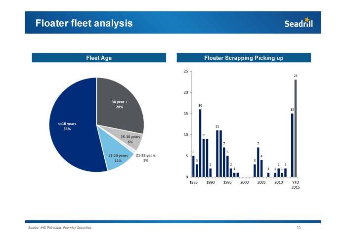
For an industry wide overview on the age of fleets see page 15 & 16 of the following Seadrill presentation, excerpted below. Nearly a third of all floater rigs are over 30 years old and over half of all jackup rigs are over 30 years old. This suggests there could be a significant number of rigs scrapped during this downturn, hopefully making the recovery all the more interesting.

010915-pareto-seadrill-ceo-presentation 15

010915-pareto-seadrill-ceo-presentation 16

I believe an interesting way to play this is via corporate debt. To give you an idea, here are some recent levels.

  1. Ensco 4.70% 3/2021    : 68 cts on the dollar
  2. Ensco 4.50% 10/2024  : 63 cts
  3. Ensco 5.20%  3/2025   :  60 cts
  4. Ensco 5.75% 10/2044   :  56 cts
  5. Diamond 5.875% 5/2019 : 90 cts
  6. Diamond 3.45% 11/2023  : 73 cts
  7. Diamond 5.70% 10/2039 : 64 cts
  8. Diamond 4.875  11/2042 :  58 cts

Disclosure – I own some of the oil rig  bonds and may purchase more.

Two great quotes ….

“History never repeats itself, but it often rhymes.” 

This quote is attributed to Mark Twain and occasionally comes to mind when considering business situations. In the early 2000s, the US steel industry was on its heels. Almost everything in the industry was distressed and bankruptcies were abundant. Into this maelstrom went bankruptcy expert Wilbur L Ross. In just a few years, he acquired and rolled up a number of bankrupt steel companies to be profitably sold to Mittal in 2005.

Is Wilbur Ross Crazy?

The Bottom-Feeder King

Fast forward to today and the quote from John F. Kennedy, the 35th President of the United States comes to mind when considering the energy sector,

“When written in Chinese, the word ‘crisis’ is composed of two characters. One represents danger and the other represents opportunity.”

I can’t help but think that someone like a Ross, a Tisch, a Zell or a Buffett will begin to do a roll up strategy acquiring high quality assets since the major oil & gas companies are too distracted by their own operations & finances to see the opportunity before them.

Case in point, Chesapeake Energy. Yes, a lot can go wrong with this company and they are paying for the sins of the forefathers, but let’s look at some basic & approximate calculations. For starters, they are the 2nd largest natural gas producer in the US.

Top 40 US natural gas producers

Conoco is #7 (Market cap $46 bio), BP (Market cap $92 bio) is #8, Chevron (Market cap $152 bio)  is #10, and Shell (Market cap $118 bio) is #18.

A “market based” enterprise value for Chesapeake = $2.3 bio (Market cap) + $5.15 bio (Market value of $11.4 bio of debt) + $3.3 bio (Minority interests & preferred shares)  – $1.759 bio (Cash) = $9.1 bio

They have 4,377,000 net acres of developed property and 3,656,000 acres of undeveloped property. Assuming the undeveloped land is only worth a quarter of the developed land value would mean the value per acre implied by the market is $9.1 bio / (4.377 mio + 0.914 mio) = $1,714 per acre of developed property and $428 per acre of undeveloped acre.

(Note – I’m unfamiliar with corporate debt and securities law around debt so take what follows with a pinch of salt. I’m just thinking out loud in areas that I have very little experience in but sense an interesting opportunity.)

These prices are significantly lower than where asset sales took place in the past. Which makes me wonder why someone with a stronger balance sheet and desire for a market leading position in natural gas production doesn’t start acquiring Chesapeake’s debt?

If an oil major were to start acquiring the debt they could either be in pole position for the assets during a bankruptcy/restructuring – or – earn a funding carry. Naturally, there’s a big caveat to this. If Chesapeake were to restructure their debt, the covenants could change or the returns diminish (maturity extended, etc.).

In the event that the majors are too preoccupied with their own company affairs, I would envisage a savy Ross, Tisch, Zell, or Buffett like player to enter with a rollup/asset acquisition strategy. Then in 3-5 years when the energy market stabilizes, they sell the entity to a major at a much higher valuation.

As I said, I’m not a credit or bankruptcy expert but the risk/reward from a countercyclical investment in shale gas assets looks as good as it gets. No?

Fromageries Bel, Lactalis & Parmalat

I stumbled upon a few interesting European cheese/dairy companies which piqued my interest in the industry and their businesses. The companies are Lactalis Group (“Lactalis”), Fromageries Bel (“Bel”) and Parmalat.  They are three separate companies with some overlap in shareholder ownership.

Fromageries Bel

Fromageries Bel is France’s third largest pure cheese producer after Lactalis (formerly Besnier) and Bongrain.  Together these three companies produce more than half of the total cheese sales in France, a country with the highest per capita consumption in the world.  You may not be familiar with Bel as a company but you are most likely familiar with their five core products – Mini Babybel®, Boursin®, Kiri®, Leerdammer®, & the Laughing Cow®.


Family business & history

The company was founded in 1865 by Jules Bel in France’s Jura region near the Swiss border. Jules Bel was joined and then succeeded by his son Léon Bel. The younger Bel was responsible for developing and registering a trademark for the Laughing Cow® cheese in 1921. In the 1930s, Léon Bel was joined by his son in law Robert Fiévet and appointed CEO in 1937. If Léon Bel had succeeded in establishing the Laughing Cow ® as successful product, Fiévet would build the company into one of the top three cheese producers in France. Then, in the 1950s their attention moved toward expansion. They reorganized, moved their headquarters to Paris and listed on the Paris Stock Exchange. By the late 1970s, a new generation entered the family-owned business, with the appointment of Bertrand Dufort, Fiévet’s son-in-law. In 1981 the company simplified its current name, to Fromageries Bel.

Interestingly enough, Bel was not alone as a market leader in the French cheese market. Another group, Besnier (today known as Lactalis), was aggressively expanding and consolidating the French dairy industry. Besnier was a private company wholly owned by the Besnier family and led by Michael Besnier. Whereas Besnier and Bongrain had developed a strong presence in the molded cheese segment, Bel had a stronghold on the melted cheese market. In 1993, Besnier began purchasing shares in Bel. By the end of 1994, Besnier (Lactalis) owned 20 percent of Bel. Bel was an easy target but the acquisition never happened.  A separate family holding company, known today as Unibel, was set up in the 1920s and was Bel’s majority shareholder.

As of today, the shareholdings in Fromagerie Bel are as follows – Unibel & family 71% , Lactalis ( formerly Besnier) 24%, Treasury shares 1.5%, Other shareholders (free float) 3.5%. Yep, that’s right. Only 3.5% of the float is available and not locked up. We’ll come back to this point later.

Lactalis

Groupe Lactalis, formerly known as Besnier, is France’s largest dairy products producer and one of the largest cheese manufacturers in the world. It ranks second in the global dairy market, after Nestle. Whereas you may never heard of the company, you will most likely be familiar with the company’s renowned President label and other brands such as Sorrento, Rondele, etc.  Lactalis is a private company 100% owned by the Besnier family.

Lactalis

Family business & history

Besnier S.A., today known as Lactalis, was founded in 1933 by Andre Besnier in Laval, in the Loire Valley region of France. Besnier remained a small, single factory operation well into the 1960s. Andre’s son, Michel Besnier, took over operations in the late 1950s with a goal to expand its operations to multiple plants and diversify the company’s dairy products. As a first step, Besnier created its own brand, the famous President Camembert label, in 1968. From the next year onwards, Michel Besnier pursued a series of acquisitions through the 1970s, 1980s, 1990s, and 2000s which catapulted the private company into the 2nd largest dairy company in the world.

http://www.lactalis.fr/english/groupe/historique.htm

Parmalat

Parmalat was founded by Calisto Tanzi in 1963 in Italy. From the start, the business pursued the expansion of new milk products which led to their flagship product – milk pasteurized at ultra-high temperatures. This was revolutionary at the time because it maintained an unrefrigerated shelf life that exceeded six months before opening. Parmalat expanded from such humble beginnings to become a large multinational firm in the late 1990s, becoming the largest Italian food company and fourth largest in Europe at the time.

Unfortunately, an accounting scandal of epic proportions was discovered in 2003 leading to Parmalat’s bankruptcy.  A new Parmalat was listed on the Italian stock exchange in October 2005.

In 2011, Lactalis bought an additional 54% of Parmalat. This took Lactalis stake in the publicly listed company to 83.3% after accounting for the 29% of the company already owned before the additional acquisition.  This means only 16.7% of the common equity is freely available. We’ll come back to this point later.

Investment thesis

I purchased shares in Fromageries Bel for the following reasons.

Financials

  • Their financials are decent. Here’s a decent CFA Society writeup on the company.
  • Solid cash flow generation allows the company to finance capital expenditures with internal financing.
  • Demonstrated long term track record of performance – delivering quality products & strong financials.

Favorable backdrop

  • Lactalis under the Besnier family appear to be an Outsider like firm which excels at acquisition and consolidation in the dairy industry.
  • Of the companies owned by Lactalis, I believe only Fromageries Bel and Parmalat are publicly listed equities but not wholly owned.
  • There is the potential for the shares not in the controlling shareholder’s hands, Lactalis’ hands, to eventually be bought out or tendered for to gain 100% ownership.

Why Fromageries Bel and not Parmalat?

I believe the incentives are better aligned in Fromageries Bel. I am working under the assumption that since Lactalis, a direct competitor, has a 24% stake in Fromageries Bel it would be hard for the Bel family or Fromageries Bel’s management to get away with any shenanigans. This counterbalance does not seem to exist amongst the shareholdings of Parmalat.

Cheese financials


A statistician’s foray in value investing

Benjamin Graham and Warren Buffett have imparted a treasure trove of knowledge on the topic of investing for the public. Reading Graham’s Intelligent Investor and Buffett’s three decades of Berkshire Hathaway’s shareholder letters is a rare treat. The reader participates in the thought process of two of the most astute investment minds of the 20th century and discovers the required temperament for long term investment success. As such, my comments down below should be viewed as someone thankful for the insights but willing to question the statements and methods, having nonetheless benefited immensely from the knowledge imparted by them through their original delivery.

Holding a central place in the teachings of Benjamin Graham, the father of value investing, is the concept of intrinsic value and margin of safety. Simply stated, intrinsic value is how much a given company is worth as a private concern in its entirety. This can be quite different from its market capitalization, which is the price Mr. Market is willing to offer the company for on a daily basis. Margin of safety, as coined by Graham, describes the extra cushion of value between the price paid for a company and the company’s intrinsic value.

Prima facie, a politician’s campaign speech to end world hunger is equally as noble, but dismissed as a mere platitude, begging the question – “Great, who wouldn’t want to do that? How do you plan on accomplishing this?” But somehow, under the aura of the investment greats, the concept of intrinsic value and margin of safety avoid such inquisitions. But wouldn’t we all want to know the value of what we’re buying and how much of a good or bad deal we’re receiving? After all, who wouldn’t want to buy 50 cent dollars? Or alternatively, who would really want to pay a dollar fifty for a dollar?

This leads us to what I believe to be the main deficiency of value investing as espoused by Graham and his acolytes. It lacks a testable hypothesis. The lack of a testable or falsifiable hypothesis is what separates astrology from astronomy, creationism from evolution and is best captured by a lengthy excerpt of Karl Popper’s, the well know Austrian-born philosopher of science, in Conjectures and Refutations : The Growth of Scientific Knowledge.

“When should a theory be ranked as scientific?” or “Is there a criterion for the scientific character or status of a theory?”

The problem which troubled me at the time was neither, “When is a theory true?” nor “When is a theory acceptable?” my problem was different. I wished to distinguish between science and pseudo-science; knowing very well that science often errs, and that pseudoscience may happen to stumble on the truth.

I knew, of course, the most widely accepted answer to my problem: that science is distinguished from pseudoscience—or from “metaphysics”— by its empirical method, which is essentially inductive, proceeding from observation or experiment. But this did not satisfy me. On the contrary, I often formulated my problem as one of distinguishing between a genuinely empirical method and a non-empirical or even pseudo- empirical method — that is to say, a method which, although it appeals to observation and experiment, nevertheless does not come up to scientific standards. The latter method may be exemplified by astrology, with its stupendous mass of empirical evidence based on observation — on horoscopes and on biographies.

These considerations led me in the winter of 1919-20 to conclusions which I may now reformulate as follows.

1.  It is easy to obtain confirmations, or verifications, for nearly every theory — if we look for confirmations.
2.  Confirmations should count only if they are the result of risky predictions; that is to say, if, unenlightened by the theory in question, we should have expected an event which was incompatible with the theory — an event which would have refuted the theory.
3.  Every “good” scientific theory is a prohibition: it forbids certain things to happen. The more a theory forbids, the better it is.
4.  A theory which is not refutable by any conceivable event is non- scientific. Irrefutability is not a virtue of a theory (as people often think) but a vice.
5.  Every genuine test of a theory is an attempt to falsify it, or to refute it. Testability is falsifiability; but there are degrees of testability: some theories are more testable, more exposed to refutation, than others; they take, as it were, greater risks.
6.  Confirming evidence should not count except when it is the result of a genuine test of the theory; and this means that it can be presented as a serious but unsuccessful attempt to falsify the theory. (I now speak in such cases of “corroborating evidence.”)
7.  Some genuinely testable theories, when found to be false, are still upheld by their admirers — for example by introducing ad hoc some auxiliary assumption, or by reinterpreting the theory ad hoc in such a way that it escapes refutation. Such a procedure is always possible, but it rescues the theory from refutation only at the price of destroying, or at least lowering, its scientific status. (I later described such a rescuing operation as a “conventionalist twist” or a “conventionalist stratagem.”)

One can sum up all this by saying that the criterion of the scientific status of a theory is its falsifiability, or refutability, or testability.

To be sure, value investing, even loosely defined as it is, is a vastly superior method to rank speculation and Graham et al are to be thanked for their contributions. Yet in order for one to believe that value investing is superior to other investment methods, one must heed the wisdom of Karl Popper and posit a testable hypothesis. A hypothesis that goes beyond the ill-defined mandate of buying 50 cent dollars, beyond the nebulous definition of intrinsic value and into the domain of a concrete, empirical and repeatable method to calculate intrinsic value and margin of safety. After all, isn’t the expression intrinsic value debased of any true meaning if we’re each allowed to have our own personal definition of this term?

In pursuit of this noble goal we are immediately beset by another setback. A testable hypothesis implies the use of cold, mechanical and quantitative methods to discern intrinsic value. But all too often, quantitative methods applied in the financial arena just lead to sophistry disguised as numerical precision. This false sense of precision did not escape either Graham or Buffett, butdoes escape many investors.

“In forty-four years of Wall Street experience and study I have never seen dependable calculations made about common-stock values, or related investment policies that went beyond simple arithmetic or the most elementary algebra. Whenever calculus is brought in, or higher algebra, you could take it as a warning signal that the operator was trying to substitute theory for experience, and usually also to give to speculation the deceptive guise of investment.”
– Benjamin Graham

Perhaps we should review the academic and investment communities’ fate in applying sophisticated quantitative models. With any luck, our review will aid in designing and testing a procedure for quantitatively determining intrinsic value as well as address the issue of precision or lack thereof.

Currently, there are two main quantitative approaches within the academic community to determine optimal portfolio allocations (1) the mean variance (MV) approach as espoused by Nobel laureate, Harry Markowitz; and (2) the arbitrage pricing theory (APT) approach as developed by Stephen Ross. Unfortunately, embedded within each paradigm are the potential seeds of the false and misleading precision that so irked Graham.

For the purely quantitative portfolio manager, Markowitz’s mean-variance framework, in theory, allows one to determine the optimal portfolio weights without any consideration for company specific information. In many ways, it is the antithesis of value investing. The portfolio manager merely focuses on the sequence of returns provided by Mr. Market and invests accordingly. This framework requires knowledge of both the mean and covariance of asset returns, which in reality are unknown and have to be estimated from the observed data. Nevertheless, standard industry practice is to ignore the estimation error and simply treat the sample estimates as the true parameters, plugging them in to get optimal portfolio weights.

In this case, Graham’s concerns about false precision are justified by the naivety in which a variable of interest’s point estimate, the mean and covariance, are used without any consideration for the variability of these estimates. Luckily, their exasperation can be alleviated by an appropriate and requisite use of statistics.

If one evaluates the repercussions of such estimation error on the investment decision at hand, an amazing empirical fact emerges. We discover that the precision we initially sought has in fact disappeared. We know with statistical certainty that our desired result is unknowable. So in the hunt for quantitative precision, we are lead to acknowledge our very own lack of precision. In fact, there is strong empirical and theoretical evidence to suggest that an equal weight portfolio will ex- ante outperform any so called Markowitz mean-variance optimal portfolio with high probability.

The second approach, the Arbitrage Pricing Theory (APT) model, decomposes a stock’s return into factors common to all assets and factors specific to a given asset. Macroeconomic factors like the inflation rate, unemployment rate and interest rates would be examples of factors common to all assets while attributes such as size, dividend yield, price momentum, book value, free cash flow, and return on equity would be examples of firm specific factors.

Once such a factor model is posited, the principled practitioner would perform a multiple regression to determine the betas for each factor and each stock. With these betas in hand, a cross sectional regression would determine which factors or exposures were being rewarded and which were not. Those stocks being highly rewarded by such priced risk factors would be purchased and those not rewarded, avoided.

The APT model shares a kindred spirit with value investing. It provides an investor with the relevant factors and a cold, mechanical and quantitative method with which to order or rank various investment opportunities, but it does not determine an intrinsic value per se.

Unfortunately, once again, Graham’s and Buffett’s apprehension of sophisticated quantitative techniques are well founded. Many practitioners blindly pursue a kitchen sink approach where they chuck in all sorts of factors in an APT model. This makes a mockery of statistics as well as a mockery of common sense. For the statistically minded, data mining, variable selection and multicollinearity are obvious problems that will relegate the regression’s factor loadings to be quite meaningless – both statistically and economically. Yet a well specified, parsimonious model with just a few factors, could lead to results that are both economically meaningful and statistical significant.

But this brings us back where we started and in an uncomfortable impasse. Clearly we need a testable theory to base our investments on, yet a carefully conducted and expansive quantitative approach will leave us with an answer that is best described by a shrug of the shoulders and an “Ughh, I don’t know.” Alternatively, a few, a priori, well chosen factors will lead to a meaningful result. But this just means if we start with qualitatively sensible factors like momentum, size, price to book, return on invested capital, free cash flow yield, and earning’s yield, then we can quantitatively arrive at a justified and defensible conclusion.

As such, value investing’s lack of a testable hypothesis does not relegate it to the wrath of financial astrology because of its a priori foundation on sound business practices and sensible qualitative factors. Some may find this impasse quite troubling but in the end, the most financially of action is to be intellectually honest with what we know, what we don’t know,
and what is unknowable.

Equity factor model – the poor man’s version.

My encounter with value investing began somewhat backwards during graduate school. I enrolled in an Empirical Finance course to satiate my curiosity on financial markets and break the monotony of math every day from dawn to dusk.

The course was intended for first year Finance PhD students and covered time-series & cross-sectional properties of asset returns, event studies, and empirical tests of asset pricing models. But for someone like myself who spent the previous ten years trading foreign exchange and commodity markets, the most interesting part of the course was when we explored the interplay between asset pricing theories, statistical assumptions and relevant econometric techniques in the context of classic empirical papers.

Quite quickly, I realized that for every theory posited, an anomaly would be discovered that highlighted the shortcomings of the various academic models. Given that it would be near heretic for an aspiring academic to say the markets were inefficient, the academic community would quickly go on to either explain why such an anomaly really wasn’t an anomaly or develop a better model of asset returns.

But for me, a practitioner who believed that there were opportunities to make reasonable returns from investing in the financial markets, it was music to my ears. The most useful research was always meticulous and grounded in a company’s fundamentals. Things like book value, cash flow, accruals, etc. Collectively, the body of research provided a useful guide as to what may or may not work in the real world and best of all, it was free, rigorous and testable.

Upon graduation, I found myself with a bit of time on my hands before I launched a cmmodity fund so I decided to read all of Warren Buffett’s shareholder letters and The Intelligent Investor by Benjamin Graham.

With this, my two worlds collided. I immediately saw the value of blending a quantitative and qualitative approach to investing. And since that time, it’s been a hobby of mine to continually read the academic research looking for ways to build simple, parsimonious and practical quantitative models to find value stocks.

The factors that I’ve landed upon to build an implementable factor model are as follows

  1. Accruals
  2. Beta
  3. EPS Estimate revisions
  4. EV / EBITDA
  5. EV / MCAP
  6. Financial leverage
  7. Goodwill/Intangible to Equity
  8. Gross margins
  9. Gross profit to total assets
  10. Growth rate of shares
  11. Growth rate of total assets
  12. Inside ownership
  13. Pretax earning yield
  14. Price to free cash flow
  15. Return on assets
  16. Scaled net operating assets
  17. Standard deviation of returns
  18. 5 year returns (mean reversion)
  19. 6 month return (momentum)

For some factors, the higher the better and for other factors, the lower the better. For each factor, there was academic research that showed the efficacy of such a factor in investing, e.g. Sloane (1996) for accruals, Jegadeesh and Titman (1993) for momentum, DeBondt and Thaler (1989) for mean reversion, etc. Over the years, I always filtered the research since most professors publish research in pursuit of tenure and not in pursuit of implementing profitable trading strategies. A good compendium of many known anomalies is Jacobs, Heiko, 2015, “What Explains the Dynamics of 100 Anomalies”, Journal of Banking and Finance, 57, 65-85.

But an important question is how do you combine all of these factors to form a composite score and appropriately deal with outliers. There are countless statistical ways to do this and a number of theories abound. I’ve thought about this long and hard and explored many of the sophisticated approaches. In the end, I think this is where the qualitative judgement of a practitioner comes in. How much should an overall score depend on the balance sheet statement? The cash flow statement? The stock price returns? These are questions best answered by the investor who will actually deploy capital and not be second guessing himself during a market pullback.

As for me, I chose to do this a few ways

  1. Just pick the weightings for each factor. All equal weight? Some more important, etc.?
  2. Create a risk-reward composite score. Average factor score to average factor variability ratio?
  3. Median factor score?
  4. Trimmed mean value of factors?
  5. Perform a regression of past returns versus past factor scores to arrive at regression coefficients for the factor scores. Once you have the regression coefficients you plug in the new factor scores to give you the composite score to rank the investment universe on.

Once the Q4  2015 financial data is available, I’ll run my model and post a list of the top companies using one of the composite scoring methods above. I normally comb through the top 200 names to see which ones warrant an investment.

Interestingly enough, what started as a curiosity about value investing over a decade ago soon became an investing hobby. What started as an investing hobby led to a fundamental shift in how I evaluate businesses, whether for investment or direct management during my time at a major bank. Warren Buffett’s quote “I am a better investor because I am a businessman, and a better businessman because I am an investor” surely resonates with me.

Chesapeake Energy

In 2008, I was on a commodities panel with three other fellow panelists at an all-day investment conference. I’ve never been one to refrain from sharing my opinion and I was running my own Commodity Trading Advisor (CTA) at the time so there was no wider corporate censure or opprobrium if I spoke freely. Sure enough, when the topic came to a Wall Street darling at the time – Aubrey McClendon and Chesapeake Energy – I let it rip. I still remember the surprise and disdainful looks I received from calling the individual and institution a bunch of cowboys trying to disguise themselves as value focused business people. Recall that in 2008, when Chesapeake’s stock plummeted, Aubrey McClendon forfeited most of his stock to a margin call because he had borrowed hundreds of millions to purchase yet more Chesapeake stock. Luckily for him, the board voted to give him a $75 million bonus to continue participating in his “Founders Well Participation Program” and also purchased his rare map collections for $12.1 million. What? Corporate governance? Hello? Does this really happen?

Back then the hype was overblown but fast forward to today and perhaps the market’s despair is overdone? Yes, commodity prices are down materially and Chesapeake has more than enough exposure to oil & gas prices but let’s review the facts.

In 2013, the founder and erstwhile CEO, Aubrey McClendon, stepped down after years of boom time growth amidst a maelstrom of media reports of conflicts of interest between himself & Chesapeake. He left Chesapeake as a highly levered firm.  Around this time, the stock collapsed and a well-known activist (Carl Icahn) and a well know value investor (Mason Hawkins) stepped in to buy large stakes of common equity.  The two investors own about 25% of the market cap in Q2 2015. Since 2013, the firm has moved to divest assets and de-leverage its balance sheet. Unfortunately, the starting point isn’t great but they have two very large advantages versus their peer group – (1) they started the fire drill exercise two years before everyone else (2) they knew they were in crisis mode from 2013 so there was no head in sand syndrome of denial. They knew they had to act and do it while the borrowing window was open.

  • Year to date, Chesapeake has taken $15 billion (yes, billion) of impairments to their balance sheet.
  • Chesapeake’s total assets hit a peak in 2012 at $47 billion but as of Q3 2015, their total assets stand at $21 billion.
  • Chesapeake’s total liabilities hit a peak in 2012 at $30 billion but as of Q3 2015, their total liabilities stand at $17 billion.
  • Free cash flow has been negative since 2006. So now they have asset sales to raise cash and impairments that cost money. Case in point — they raise cash in 2014 and announce a $5 billion impairment charge in 2015.

Will they get out of the mess? Not sure. It’s far from a no brainer and maybe it’s more of an even odds bet…but they’ve done a few interesting things lately around their debt to extend their weighted maturities so it could be interesting. I’ve gone ahead and purchased a bit of the 4.5% Cumulative Convertible Preferred on Chesapeake (unfortunately at a higher price than current levels). The current price is at distress levels with a current yield around 26%. It’s pricing in disaster so who knows, maybe it goes lower or maybe it just works out ok.  Either way, it’ll pretty interesting to follow and see how the various interested parties play the game – existing management, common equity holders, and debt holders.